|
Supplementary code for the Build a Large Language Model From Scratch book by Sebastian Raschka Code repository: https://github.com/rasbt/LLMs-from-scratch |

|
Appendix D: Adding Bells and Whistles to the Training Loop#
In this appendix, we add a few more advanced features to the training function, which are used in typical pretraining and finetuning; finetuning is covered in chapters 6 and 7
The next three sections below discuss learning rate warmup, cosine decay, and gradient clipping
The final section adds these techniques to the training function
We start by initializing a model reusing the code from chapter 5:
from importlib.metadata import version
import torch

print("torch version:", version("torch"))


from previous_chapters import GPTModel
# If the `previous_chapters.py` file is not available locally,
# you can import it from the `llms-from-scratch` PyPI package.
# For details, see: https://github.com/rasbt/LLMs-from-scratch/tree/main/pkg
# E.g.,
# from llms_from_scratch.ch04 import GPTModel

GPT_CONFIG_124M = {
    "vocab_size": 50257,   # Vocabulary size
    "context_length": 256, # Shortened context length (orig: 1024)
    "emb_dim": 768,        # Embedding dimension
    "n_heads": 12,         # Number of attention heads
    "n_layers": 12,        # Number of layers
    "drop_rate": 0.1,      # Dropout rate
    "qkv_bias": False      # Query-key-value bias
}

device = torch.device("cuda" if torch.cuda.is_available() else "cpu")

# Note:
# Uncommenting the following lines will allow the code to run on Apple Silicon chips, if applicable,
# which is approximately 2x faster than on an Apple CPU (as measured on an M3 MacBook Air).
# However, the resulting loss values may be slightly different.

#if torch.cuda.is_available():
#    device = torch.device("cuda")
#elif torch.backends.mps.is_available():
#    device = torch.device("mps")
#else:
#    device = torch.device("cpu")
#
# print(f"Using {device} device.")

torch.manual_seed(123)
model = GPTModel(GPT_CONFIG_124M)
model.eval();  # Disable dropout during inference
---------------------------------------------------------------------------
ModuleNotFoundError                       Traceback (most recent call last)
Cell In[1], line 2
      1 from importlib.metadata import version
----> 2 import torch
      4 print("torch version:", version("torch"))
      7 from previous_chapters import GPTModel

ModuleNotFoundError: No module named 'torch'
Next, using the same code we used in chapter 5, we initialize the data loaders:
import os
import urllib.request

file_path = "the-verdict.txt"
url = "https://raw.githubusercontent.com/rasbt/LLMs-from-scratch/main/ch02/01_main-chapter-code/the-verdict.txt"

if not os.path.exists(file_path):
    with urllib.request.urlopen(url) as response:
        text_data = response.read().decode('utf-8')
    with open(file_path, "w", encoding="utf-8") as file:
        file.write(text_data)
else:
    with open(file_path, "r", encoding="utf-8") as file:
        text_data = file.read()
from previous_chapters import create_dataloader_v1
# Alternatively:
# from llms_from_scratch.ch02 import create_dataloader_v1


# Train/validation ratio
train_ratio = 0.90
split_idx = int(train_ratio * len(text_data))


torch.manual_seed(123)

train_loader = create_dataloader_v1(
    text_data[:split_idx],
    batch_size=2,
    max_length=GPT_CONFIG_124M["context_length"],
    stride=GPT_CONFIG_124M["context_length"],
    drop_last=True,
    shuffle=True,
    num_workers=0
)

val_loader = create_dataloader_v1(
    text_data[split_idx:],
    batch_size=2,
    max_length=GPT_CONFIG_124M["context_length"],
    stride=GPT_CONFIG_124M["context_length"],
    drop_last=False,
    shuffle=False,
    num_workers=0
)
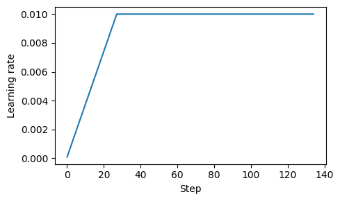
D.1 Learning rate warmup#
When training complex models like LLMs, implementing learning rate warmup can help stabilize the training
In learning rate warmup, we gradually increase the learning rate from a very low value (
initial_lr) to a user-specified maximum (peak_lr)This way, the model will start the training with small weight updates, which helps decrease the risk of large destabilizing updates during the training
n_epochs = 15
initial_lr = 0.0001
peak_lr = 0.01
Typically, the number of warmup steps is between 0.1% to 20% of the total number of steps
We can compute the increment as the difference between the
peak_lrandinitial_lrdivided by the number of warmup steps
total_steps = len(train_loader) * n_epochs
warmup_steps = int(0.2 * total_steps) # 20% warmup
print(warmup_steps)
27
Note that the print book accidentally includes a leftover code line,
warmup_steps = 20, which is not used and can be safely ignored
lr_increment = (peak_lr - initial_lr) / warmup_steps

global_step = -1
track_lrs = []

optimizer = torch.optim.AdamW(model.parameters(), weight_decay=0.1)

for epoch in range(n_epochs):
    for input_batch, target_batch in train_loader:
        optimizer.zero_grad()
        global_step += 1

        if global_step < warmup_steps:
            lr = initial_lr + global_step * lr_increment
        else:
            lr = peak_lr

        # Apply the calculated learning rate to the optimizer
        for param_group in optimizer.param_groups:
            param_group["lr"] = lr
        track_lrs.append(optimizer.param_groups[0]["lr"])

        # Calculate loss and update weights
        # ...
import matplotlib.pyplot as plt

plt.figure(figsize=(5, 3))
plt.ylabel("Learning rate")
plt.xlabel("Step")
total_training_steps = len(train_loader) * n_epochs
plt.plot(range(total_training_steps), track_lrs)
plt.tight_layout(); plt.savefig("1.pdf")
plt.show()
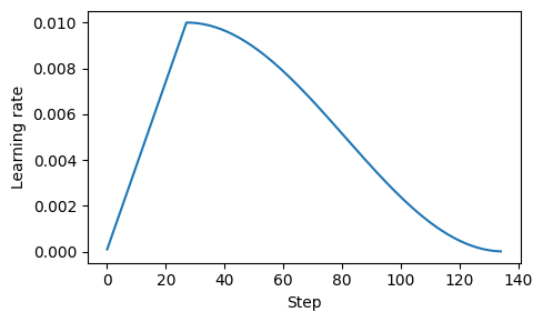
D.2 Cosine decay#
Another popular technique for training complex deep neural networks is cosine decay, which also adjusts the learning rate across training epochs
In cosine decay, the learning rate follows a cosine curve, decreasing from its initial value to near zero following a half-cosine cycle
This gradual reduction is designed to slow the pace of learning as the model begins to improve its weights; it reduces the risk of overshooting minima as the training progresses, which is crucial for stabilizing the training in its later stages
Cosine decay is often preferred over linear decay for its smoother transition in learning rate adjustments, but linear decay is also used in practice (for example, OLMo: Accelerating the Science of Language Models)
import math

min_lr = 0.1 * initial_lr
track_lrs = []

lr_increment = (peak_lr - initial_lr) / warmup_steps
global_step = -1

for epoch in range(n_epochs):
    for input_batch, target_batch in train_loader:
        optimizer.zero_grad()
        global_step += 1

        # Adjust the learning rate based on the current phase (warmup or cosine annealing)
        if global_step < warmup_steps:
            # Linear warmup
            lr = initial_lr + global_step * lr_increment
        else:
            # Cosine annealing after warmup
            progress = ((global_step - warmup_steps) /
                        (total_training_steps - warmup_steps))
            lr = min_lr + (peak_lr - min_lr) * 0.5 * (
                1 + math.cos(math.pi * progress))

        # Apply the calculated learning rate to the optimizer
        for param_group in optimizer.param_groups:
            param_group["lr"] = lr
        track_lrs.append(optimizer.param_groups[0]["lr"])

        # Calculate loss and update weights
plt.figure(figsize=(5, 3))
plt.ylabel("Learning rate")
plt.xlabel("Step")
plt.plot(range(total_training_steps), track_lrs)
plt.tight_layout(); plt.savefig("2.pdf")
plt.show()
D.3 Gradient clipping#
Gradient clipping is yet another technique used to stabilize the training when training LLMs
By setting a threshold, gradients exceeding this limit are scaled down to a maximum magnitude to ensure that the updates to the model’s parameters during backpropagation remain within a manageable range
For instance, using the
max_norm=1.0setting in PyTorch’sclip_grad_norm_method means that the norm of the gradients is clipped such that their maximum norm does not exceed 1.0the “norm” refers to a measure of the gradient vector’s length (or magnitude) in the parameter space of the model
Specifically, it’s the L2 norm, also known as the Euclidean norm
Mathematically, for a vector \(\mathbf{v}\) with components \(\mathbf{v} = [v_1, v_2, \ldots, v_n]\), the L2 norm is defined as: $\( \| \mathbf{v} \|_2 = \sqrt{v_1^2 + v_2^2 + \ldots + v_n^2} \)$
The L2 norm is calculated similarly for matrices.
Let’s assume our gradient matrix is: $\( G = \begin{bmatrix} 1 & 2 \\ 2 & 4 \end{bmatrix} \)$
And we want to clip these gradients with a
max_normof 1.First, we calculate the L2 norm of these gradients: $\( \|G\|_2 = \sqrt{1^2 + 2^2 + 2^2 + 4^2} = \sqrt{25} = 5 \)$
Since \(\|G\|_2 = 5\) is greater than our
max_normof 1, we need to scale down the gradients so that their norm is exactly 1. The scaling factor is calculated as \(\frac{max\_norm}{\|G\|_2} = \frac{1}{5}\).Therefore, the scaled gradient matrix \(G'\) will be as follows: $\( G' = \frac{1}{5} \times G = \begin{bmatrix} \frac{1}{5} & \frac{2}{5} \\ \frac{2}{5} & \frac{4}{5} \end{bmatrix} \)$
Let’s see this in action
First, we initialize a new model and calculate the loss for a training batch like we would do in the regular training loop
from previous_chapters import calc_loss_batch
# Alternatively:
# from llms_from_scratch.ch05 import calc_loss_batch


torch.manual_seed(123)
model = GPTModel(GPT_CONFIG_124M)
model.to(device)

loss = calc_loss_batch(input_batch, target_batch, model, device)
loss.backward()
If we call
.backward(), PyTorch will calculate the gradients and store them in a.gradattribute for each weight (parameter) matrixLet’s define a utility function to calculate the highest gradient based on all model weights
def find_highest_gradient(model):
    max_grad = None
    for param in model.parameters():
        if param.grad is not None:
            grad_values = param.grad.data.flatten()
            max_grad_param = grad_values.max()
            if max_grad is None or max_grad_param > max_grad:
                max_grad = max_grad_param
    return max_grad

print(find_highest_gradient(model))
tensor(0.0411)
Applying gradient clipping, we can see that the largest gradient is now substantially smaller:
torch.nn.utils.clip_grad_norm_(model.parameters(), max_norm=1.0)
print(find_highest_gradient(model))
tensor(0.0185)
D.4 The modified training function#
Now let’s add the three concepts covered above (learning rate warmup, cosine decay, and gradient clipping) to the
train_model_simplefunction covered in chapter 5 to create the more sophisticatedtrain_modelfunction below:
from previous_chapters import evaluate_model, generate_and_print_sample
# Alternatively:
# from llms_from_scratch.ch05 import evaluate_model, generate_and_print_samplee


ORIG_BOOK_VERSION = False


def train_model(model, train_loader, val_loader, optimizer, device,
                n_epochs, eval_freq, eval_iter, start_context, tokenizer,
                warmup_steps, initial_lr=3e-05, min_lr=1e-6):

    train_losses, val_losses, track_tokens_seen, track_lrs = [], [], [], []
    tokens_seen, global_step = 0, -1

    # Retrieve the maximum learning rate from the optimizer
    peak_lr = optimizer.param_groups[0]["lr"]

    # Calculate the total number of iterations in the training process
    total_training_steps = len(train_loader) * n_epochs

    # Calculate the learning rate increment during the warmup phase
    lr_increment = (peak_lr - initial_lr) / warmup_steps

    for epoch in range(n_epochs):
        model.train()
        for input_batch, target_batch in train_loader:
            optimizer.zero_grad()
            global_step += 1

            # Adjust the learning rate based on the current phase (warmup or cosine annealing)
            if global_step < warmup_steps:
                # Linear warmup
                lr = initial_lr + global_step * lr_increment
            else:
                # Cosine annealing after warmup
                progress = ((global_step - warmup_steps) /
                            (total_training_steps - warmup_steps))
                lr = min_lr + (peak_lr - min_lr) * 0.5 * (1 + math.cos(math.pi * progress))

            # Apply the calculated learning rate to the optimizer
            for param_group in optimizer.param_groups:
                param_group["lr"] = lr
            track_lrs.append(lr)  # Store the current learning rate

            # Calculate and backpropagate the loss
            loss = calc_loss_batch(input_batch, target_batch, model, device)
            loss.backward()

            # Apply gradient clipping after the warmup phase to avoid exploding gradients
            if ORIG_BOOK_VERSION:
                if global_step > warmup_steps:
                    torch.nn.utils.clip_grad_norm_(model.parameters(), max_norm=1.0)
            else:
                if global_step >= warmup_steps:  # the book originally used global_step > warmup_steps, which lead to a skipped clipping step after warmup
                    torch.nn.utils.clip_grad_norm_(model.parameters(), max_norm=1.0)

            optimizer.step()
            tokens_seen += input_batch.numel()

            # Periodically evaluate the model on the training and validation sets
            if global_step % eval_freq == 0:
                train_loss, val_loss = evaluate_model(
                    model, train_loader, val_loader,
                    device, eval_iter
                )
                train_losses.append(train_loss)
                val_losses.append(val_loss)
                track_tokens_seen.append(tokens_seen)
                # Print the current losses
                print(f"Ep {epoch+1} (Iter {global_step:06d}): "
                      f"Train loss {train_loss:.3f}, "
                      f"Val loss {val_loss:.3f}"
                )

        # Generate and print a sample from the model to monitor progress
        generate_and_print_sample(
            model, tokenizer, device, start_context
        )

    return train_losses, val_losses, track_tokens_seen, track_lrs
import tiktoken

# Note:
# Uncomment the following code to calculate the execution time
# import time
# start_time = time.time()

torch.manual_seed(123)
model = GPTModel(GPT_CONFIG_124M)
model.to(device)

peak_lr = 0.001  # this was originally set to 5e-4 in the book by mistake
optimizer = torch.optim.AdamW(model.parameters(), lr=peak_lr, weight_decay=0.1)  # the book accidentally omitted the lr assignment
tokenizer = tiktoken.get_encoding("gpt2")

n_epochs = 15
train_losses, val_losses, tokens_seen, lrs = train_model(
    model, train_loader, val_loader, optimizer, device, n_epochs=n_epochs,
    eval_freq=5, eval_iter=1, start_context="Every effort moves you",
    tokenizer=tokenizer, warmup_steps=warmup_steps,
    initial_lr=1e-5, min_lr=1e-5
)

# Note:
# Uncomment the following code to show the execution time
# end_time = time.time()
# execution_time_minutes = (end_time - start_time) / 60
# print(f"Training completed in {execution_time_minutes:.2f} minutes.")
Ep 1 (Iter 000000): Train loss 10.934, Val loss 10.939
Ep 1 (Iter 000005): Train loss 9.151, Val loss 9.461
Every effort moves you,,,,,,,,,,,,,,,,,,,,,,,,,,,,,,,,,,,,,,,,,,,,,,,,,,
Ep 2 (Iter 000010): Train loss 7.949, Val loss 8.184
Ep 2 (Iter 000015): Train loss 6.362, Val loss 6.876
Every effort moves you,,,,,,,,,,,,,,,,,,, the,,,,,,,,, the,,,,,,,,,,, the,,,,,,,,
Ep 3 (Iter 000020): Train loss 5.851, Val loss 6.607
Ep 3 (Iter 000025): Train loss 5.750, Val loss 6.634
Every effort moves you. "I"I and I had to the to the to the and the of the to the of the to Gisburn, and the of the the of the of the to the to the of the of the of the to the of
Ep 4 (Iter 000030): Train loss 4.617, Val loss 6.714
Ep 4 (Iter 000035): Train loss 4.277, Val loss 6.640
Every effort moves you, I was. Gisburn. Gisburn's. Gisburn. Gisburn's of the of Jack's. "I of his I had the of the of the of his of, I had been. I was.
Ep 5 (Iter 000040): Train loss 3.194, Val loss 6.324
Every effort moves you know the, and in the picture--I he said, the picture--his, so--his, and the, and, and, in the, the picture, and, and, and as he said, and--because he had been his
Ep 6 (Iter 000045): Train loss 2.488, Val loss 6.263
Ep 6 (Iter 000050): Train loss 2.627, Val loss 6.264
Every effort moves you in the inevitable garlanded frame.
Ep 7 (Iter 000055): Train loss 2.193, Val loss 6.201
Ep 7 (Iter 000060): Train loss 0.818, Val loss 6.340
Every effort moves you know," was one of the picture for nothing--I told Mrs.  "I looked--I looked up, I felt to see a smile behind his close grayish beard--as if he had the donkey, and were amusing himself by holding
Ep 8 (Iter 000065): Train loss 0.735, Val loss 6.329
Ep 8 (Iter 000070): Train loss 0.789, Val loss 6.390
Every effort moves you?"  "Yes--quite insensible to the irony. She wanted him vindicated--and by me!"  He laughed again, and threw back his head to look up at the sketch of the donkey. "There were days when I
Ep 9 (Iter 000075): Train loss 0.293, Val loss 6.508
Ep 9 (Iter 000080): Train loss 0.224, Val loss 6.647
Every effort moves you?"  "Yes--quite insensible to the irony. She wanted him vindicated--and by me!"  He laughed again, and threw back his head to look up at the sketch of the donkey. "There were days when I
Ep 10 (Iter 000085): Train loss 0.234, Val loss 6.746
Every effort moves you?"  "Yes--quite insensible to the irony. She wanted him vindicated--and by me!"  He laughed again, and threw back his head to look up at the sketch of the donkey. "There were days when I
Ep 11 (Iter 000090): Train loss 0.139, Val loss 6.827
Ep 11 (Iter 000095): Train loss 0.093, Val loss 6.828
Every effort moves you?"  "Yes--quite insensible to the irony. She wanted him vindicated--and by me!"  He laughed again, and threw back his head to look up at the sketch of the donkey. "There were days when I
Ep 12 (Iter 000100): Train loss 0.057, Val loss 6.884
Ep 12 (Iter 000105): Train loss 0.071, Val loss 6.917
Every effort moves you?"  "Yes--quite insensible to the irony. She wanted him vindicated--and by me!"  He laughed again, and threw back his head to look up at the sketch of the donkey. "There were days when I
Ep 13 (Iter 000110): Train loss 0.039, Val loss 6.937
Ep 13 (Iter 000115): Train loss 0.032, Val loss 6.937
Every effort moves you?"  "Yes--quite insensible to the irony. She wanted him vindicated--and by me!"  He laughed again, and threw back his head to look up at the sketch of the donkey. "There were days when I
Ep 14 (Iter 000120): Train loss 0.032, Val loss 6.934
Ep 14 (Iter 000125): Train loss 0.035, Val loss 6.936
Every effort moves you?"  "Yes--quite insensible to the irony. She wanted him vindicated--and by me!"  He laughed again, and threw back his head to look up at the sketch of the donkey. "There were days when I
Ep 15 (Iter 000130): Train loss 0.035, Val loss 6.938
Every effort moves you?"  "Yes--quite insensible to the irony. She wanted him vindicated--and by me!"  He laughed again, and threw back his head to look up at the sketch of the donkey. "There were days when I
Looking at the results above, we can see that the model starts out generating incomprehensible strings of words, whereas, towards the end, it’s able to produce grammatically more or less correct sentences
If we were to check a few passages it writes towards the end, we would find that they are contained in the training set verbatim – it simply memorizes the training data
Note that the overfitting here occurs because we have a very, very small training set, and we iterate over it so many times
The LLM training here primarily serves educational purposes; we mainly want to see that the model can learn to produce coherent text
Instead of spending weeks or months on training this model on vast amounts of expensive hardware, we load the pretrained weights
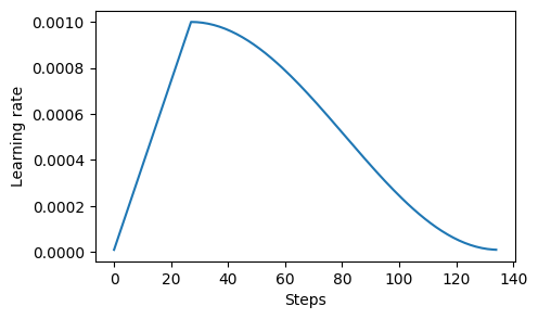
A quick check that the learning rate behaves as intended
plt.figure(figsize=(5, 3))
plt.plot(range(len(lrs)), lrs)
plt.ylabel("Learning rate")
plt.xlabel("Steps")
plt.show()
And a quick look at the loss curves
from previous_chapters import plot_losses
# Alternatively:
# from llms_from_scratch.ch05 import plot_losses


epochs_tensor = torch.linspace(1, n_epochs, len(train_losses))
plot_losses(epochs_tensor, tokens_seen, train_losses, val_losses)
plt.tight_layout(); plt.savefig("3.pdf")
plt.show()
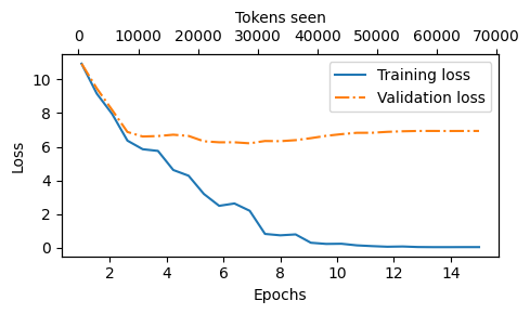
Note that the model is overfitting here because the dataset is kept very small for educational purposes (so that the code can be executed on a laptop computer)
For a longer pretraining run on a much larger dataset, see ../../ch05/03_bonus_pretraining_on_gutenberg