|
Supplementary code for the Build a Large Language Model From Scratch book by Sebastian Raschka Code repository: https://github.com/rasbt/LLMs-from-scratch |

|
Appendix E: Parameter-efficient Finetuning with LoRA#
from importlib.metadata import version

pkgs = ["matplotlib",
        "numpy",
        "tiktoken",
        "torch",
        "tensorflow", # For OpenAI's pretrained weights
        "pandas"      # Dataset loading
       ]
for p in pkgs:
    print(f"{p} version: {version(p)}")
---------------------------------------------------------------------------
PackageNotFoundError                      Traceback (most recent call last)
Cell In[1], line 11
      3 pkgs = ["matplotlib",
      4         "numpy",
      5         "tiktoken",
   (...)
      8         "pandas"      # Dataset loading
      9        ]
     10 for p in pkgs:
---> 11     print(f"{p} version: {version(p)}")

File /Library/Frameworks/Python.framework/Versions/3.10/lib/python3.10/importlib/metadata/__init__.py:946, in version(distribution_name)
    939 def version(distribution_name):
    940     """Get the version string for the named package.
    941
    942     :param distribution_name: The name of the distribution package to query.
    943     :return: The version string for the package as defined in the package's
    944         "Version" metadata key.
    945     """
--> 946     return distribution(distribution_name).version

File /Library/Frameworks/Python.framework/Versions/3.10/lib/python3.10/importlib/metadata/__init__.py:919, in distribution(distribution_name)
    913 def distribution(distribution_name):
    914     """Get the ``Distribution`` instance for the named package.
    915
    916     :param distribution_name: The name of the distribution package as a string.
    917     :return: A ``Distribution`` instance (or subclass thereof).
    918     """
--> 919     return Distribution.from_name(distribution_name)

File /Library/Frameworks/Python.framework/Versions/3.10/lib/python3.10/importlib/metadata/__init__.py:518, in Distribution.from_name(cls, name)
    516         return dist
    517 else:
--> 518     raise PackageNotFoundError(name)

PackageNotFoundError: No package metadata was found for matplotlib
E.1 Introduction to LoRA#
No code in this section
Low-rank adaptation (LoRA) is a machine learning technique that modifies a pretrained model to better suit a specific, often smaller, dataset by adjusting only a small, low-rank subset of the model’s parameters
This approach is important because it allows for efficient finetuning of large models on task-specific data, significantly reducing the computational cost and time required for finetuning
Suppose we have a large weight matrix \(W\) for a given layer
During backpropagation, we learn a \(\Delta W\) matrix, which contains information on how much we want to update the original weights to minimize the loss function during training
In regular training and finetuning, the weight update is defined as follows:
The LoRA method proposed by Hu et al. offers a more efficient alternative to computing the weight updates \(\Delta W\) by learning an approximation of it, \(\Delta W \approx AB\).
In other words, in LoRA, we have the following, where \(A\) and \(B\) are two small weight matrices:
The figure below illustrates these formulas for full finetuning and LoRA side by side
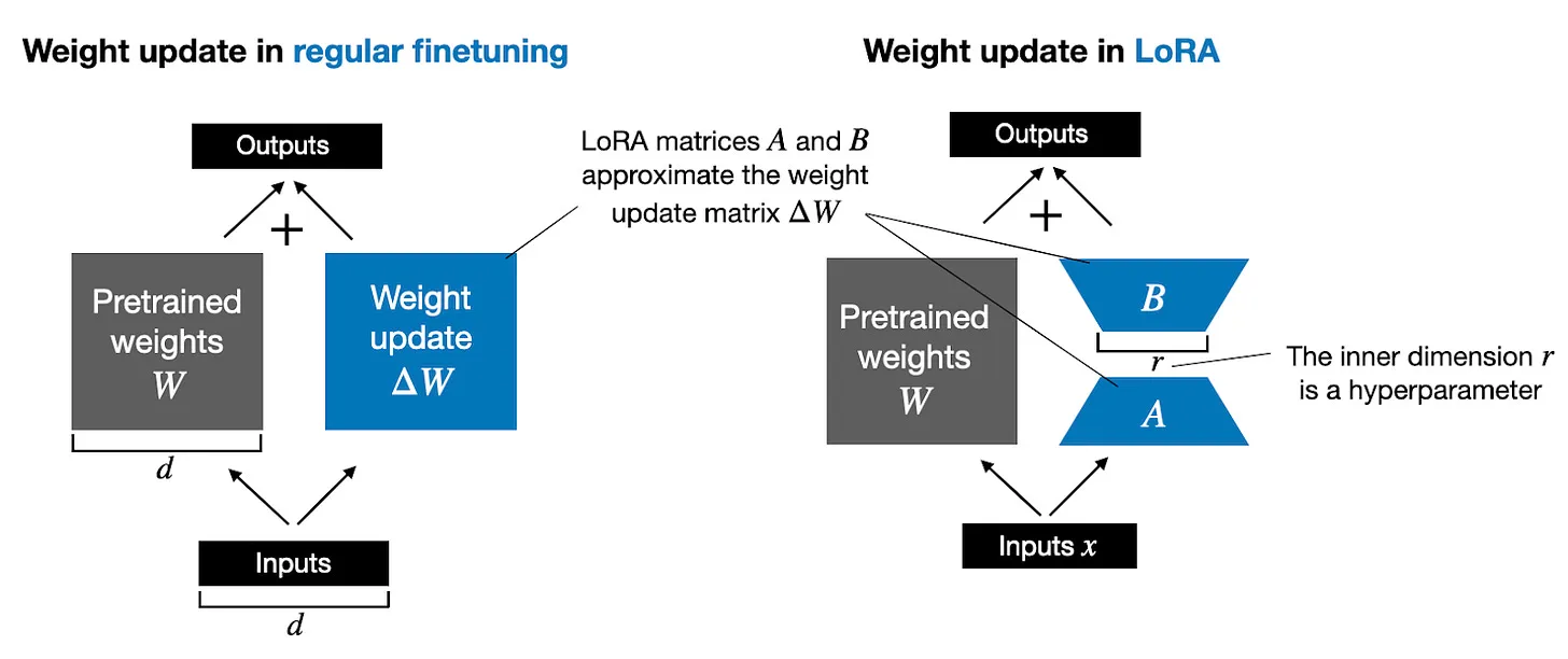
If you paid close attention, the full finetuning and LoRA depictions in the figure above look slightly different from the formulas I have shown earlier
That’s due to the distributive law of matrix multiplication: we don’t have to add the weights with the updated weights but can keep them separate
For instance, if \(x\) is the input data, then we can write the following for regular finetuning:
Similarly, we can write the following for LoRA:
The fact that we can keep the LoRA weight matrices separate makes LoRA especially attractive
In practice, this means that we don’t have to modify the weights of the pretrained model at all, as we can apply the LoRA matrices on the fly
After setting up the dataset and loading the model, we will implement LoRA in the code to make these concepts less abstract
E.2 Preparing the dataset#
This section repeats the code from chapter 6 to load and prepare the dataset
Instead of repeating this code, one could open and run the chapter 6 notebook and then insert the LoRA code from section E.4 there
(The LoRA code was originally the last section of chapter 6 but was moved to the appendix due to the length of chapter 6)
In a similar fashion, we could also apply LoRA to the models in chapter 7 for instruction finetuning
import urllib
from pathlib import Path
import pandas as pd
from previous_chapters import (
    download_and_unzip_spam_data,
    create_balanced_dataset,
    random_split
)
# If the `previous_chapters.py` file is not available locally,
# you can import it from the `llms-from-scratch` PyPI package.
# For details, see: https://github.com/rasbt/LLMs-from-scratch/tree/main/pkg
# E.g.,
# from llms_from_scratch.ch06 import (
#     download_and_unzip_spam_data,
#     create_balanced_dataset,
#     random_split
# )


url = "https://archive.ics.uci.edu/static/public/228/sms+spam+collection.zip"
zip_path = "sms_spam_collection.zip"
extracted_path = "sms_spam_collection"
data_file_path = Path(extracted_path) / "SMSSpamCollection.tsv"

try:
    download_and_unzip_spam_data(url, zip_path, extracted_path, data_file_path)
except (urllib.error.HTTPError, urllib.error.URLError, TimeoutError) as e:
    print(f"Primary URL failed: {e}. Trying backup URL...")
    url = "https://f001.backblazeb2.com/file/LLMs-from-scratch/sms%2Bspam%2Bcollection.zip"
    download_and_unzip_spam_data(url, zip_path, extracted_path, data_file_path)

df = pd.read_csv(data_file_path, sep="\t", header=None, names=["Label", "Text"])
balanced_df = create_balanced_dataset(df)
balanced_df["Label"] = balanced_df["Label"].map({"ham": 0, "spam": 1})

train_df, validation_df, test_df = random_split(balanced_df, 0.7, 0.1)
train_df.to_csv("train.csv", index=None)
validation_df.to_csv("validation.csv", index=None)
test_df.to_csv("test.csv", index=None)
File downloaded and saved as sms_spam_collection/SMSSpamCollection.tsv
import torch
import tiktoken
from previous_chapters import SpamDataset


tokenizer = tiktoken.get_encoding("gpt2")
train_dataset = SpamDataset("train.csv", max_length=None, tokenizer=tokenizer)
val_dataset = SpamDataset("validation.csv", max_length=train_dataset.max_length, tokenizer=tokenizer)
test_dataset = SpamDataset("test.csv", max_length=train_dataset.max_length, tokenizer=tokenizer)
from torch.utils.data import DataLoader

num_workers = 0
batch_size = 8

torch.manual_seed(123)

train_loader = DataLoader(
    dataset=train_dataset,
    batch_size=batch_size,
    shuffle=True,
    num_workers=num_workers,
    drop_last=True,
)

val_loader = DataLoader(
    dataset=val_dataset,
    batch_size=batch_size,
    num_workers=num_workers,
    drop_last=False,
)

test_loader = DataLoader(
    dataset=test_dataset,
    batch_size=batch_size,
    num_workers=num_workers,
    drop_last=False,
)
As a verification step, we iterate through the data loaders and check that the batches contain 8 training examples each, where each training example consists of 120 tokens
print("Train loader:")
for input_batch, target_batch in train_loader:
    pass

print("Input batch dimensions:", input_batch.shape)
print("Label batch dimensions", target_batch.shape)
Train loader:
Input batch dimensions: torch.Size([8, 120])
Label batch dimensions torch.Size([8])
Lastly, let’s print the total number of batches in each dataset
print(f"{len(train_loader)} training batches")
print(f"{len(val_loader)} validation batches")
print(f"{len(test_loader)} test batches")
130 training batches
19 validation batches
38 test batches
E.3 Initializing the model#
This section repeats the code from chapter 6 to load and prepare the model
from gpt_download import download_and_load_gpt2
from previous_chapters import GPTModel, load_weights_into_gpt
# Alternatively:
# from llms_from_scratch.ch04 import GPTModel
# from llms_from_scratch.ch05 import load_weights_into_gpt


CHOOSE_MODEL = "gpt2-small (124M)"
INPUT_PROMPT = "Every effort moves"

BASE_CONFIG = {
    "vocab_size": 50257,     # Vocabulary size
    "context_length": 1024,  # Context length
    "drop_rate": 0.0,        # Dropout rate
    "qkv_bias": True         # Query-key-value bias
}

model_configs = {
    "gpt2-small (124M)": {"emb_dim": 768, "n_layers": 12, "n_heads": 12},
    "gpt2-medium (355M)": {"emb_dim": 1024, "n_layers": 24, "n_heads": 16},
    "gpt2-large (774M)": {"emb_dim": 1280, "n_layers": 36, "n_heads": 20},
    "gpt2-xl (1558M)": {"emb_dim": 1600, "n_layers": 48, "n_heads": 25},
}

BASE_CONFIG.update(model_configs[CHOOSE_MODEL])

model_size = CHOOSE_MODEL.split(" ")[-1].lstrip("(").rstrip(")")
settings, params = download_and_load_gpt2(model_size=model_size, models_dir="gpt2")

model = GPTModel(BASE_CONFIG)
load_weights_into_gpt(model, params)
model.eval();
checkpoint: 100%|███████████████████████████| 77.0/77.0 [00:00<00:00, 45.0kiB/s]
encoder.json: 100%|███████████████████████| 1.04M/1.04M [00:00<00:00, 2.15MiB/s]
hparams.json: 100%|█████████████████████████| 90.0/90.0 [00:00<00:00, 54.5kiB/s]
model.ckpt.data-00000-of-00001: 100%|███████| 498M/498M [01:12<00:00, 6.86MiB/s]
model.ckpt.index: 100%|███████████████████| 5.21k/5.21k [00:00<00:00, 2.99MiB/s]
model.ckpt.meta: 100%|██████████████████████| 471k/471k [00:00<00:00, 1.32MiB/s]
vocab.bpe: 100%|████████████████████████████| 456k/456k [00:00<00:00, 1.48MiB/s]
To ensure that the model was loaded corrected, let’s double-check that it generates coherent text
from previous_chapters import (
    generate_text_simple,
    text_to_token_ids,
    token_ids_to_text
)


text_1 = "Every effort moves you"

token_ids = generate_text_simple(
    model=model,
    idx=text_to_token_ids(text_1, tokenizer),
    max_new_tokens=15,
    context_size=BASE_CONFIG["context_length"]
)

print(token_ids_to_text(token_ids, tokenizer))
Every effort moves you forward.

The first step is to understand the importance of your work
Then, we prepare the model for classification finetuning similar to chapter 6, where we replace the output layer
torch.manual_seed(123)

num_classes = 2
model.out_head = torch.nn.Linear(in_features=768, out_features=num_classes)
device = torch.device("cuda" if torch.cuda.is_available() else "cpu")

# Note:
# Uncommenting the following lines will allow the code to run on Apple Silicon chips, if applicable,
# which is approximately 1.2x faster than on an Apple CPU (as measured on an M3 MacBook Air).
# However, the resulting loss values may be slightly different.

#if torch.cuda.is_available():
#    device = torch.device("cuda")
#elif torch.backends.mps.is_available():
#    device = torch.device("mps")
#else:
#    device = torch.device("cpu")
#
# print(f"Using {device} device.")

model.to(device);  # no assignment model = model.to(device) necessary for nn.Module classes
Lastly, let’s calculate the initial classification accuracy of the non-finetuned model (we expect this to be around 50%, which means that the model is not able to distinguish between spam and non-spam messages yet reliably)
from previous_chapters import calc_accuracy_loader
# Alternatively:
# from llms_from_scratch.ch06 import calc_accuracy_loader


torch.manual_seed(123)
train_accuracy = calc_accuracy_loader(train_loader, model, device, num_batches=10)
val_accuracy = calc_accuracy_loader(val_loader, model, device, num_batches=10)
test_accuracy = calc_accuracy_loader(test_loader, model, device, num_batches=10)

print(f"Training accuracy: {train_accuracy*100:.2f}%")
print(f"Validation accuracy: {val_accuracy*100:.2f}%")
print(f"Test accuracy: {test_accuracy*100:.2f}%")
Training accuracy: 46.25%
Validation accuracy: 45.00%
Test accuracy: 48.75%
E.4 Parameter-efficient finetuning with LoRA#
We begin by initializing a LoRALayer that creates the matrices \(A\) and \(B\), along with the
alphascaling hyperparameter and therank(\(r\)) hyperparametersThis layer can accept an input and compute the corresponding output, as illustrated in the figure below
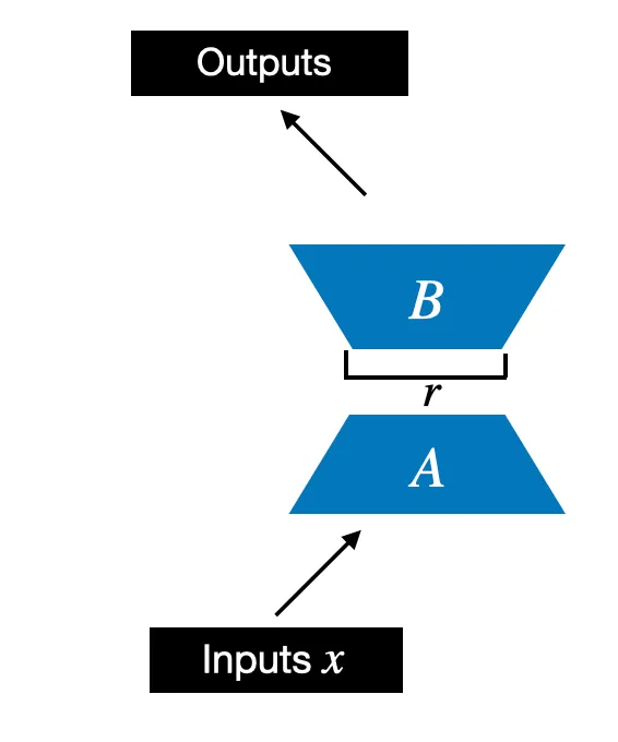
In code, this LoRA layer depicted in the figure above looks like as follows
import math

class LoRALayer(torch.nn.Module):
    def __init__(self, in_dim, out_dim, rank, alpha):
        super().__init__()
        self.A = torch.nn.Parameter(torch.empty(in_dim, rank))
        torch.nn.init.kaiming_uniform_(self.A, a=math.sqrt(5))  # similar to standard weight initialization
        self.B = torch.nn.Parameter(torch.zeros(rank, out_dim))
        self.alpha = alpha

    def forward(self, x):
        x = self.alpha * (x @ self.A @ self.B)
        return x
In the code above,
rankis a hyperparameter that controls the inner dimension of the matrices \(A\) and \(B\)In other words, this parameter controls the number of additional parameters introduced by LoRA and is a key factor in determining the balance between model adaptability and parameter efficiency
The second hyperparameter,
alpha, is a scaling hyperparameter applied to the output of the low-rank adaptationIt essentially controls the extent to which the adapted layer’s output is allowed to influence the original output of the layer being adapted
This can be seen as a way to regulate the impact of the low-rank adaptation on the layer’s output
So far, the
LoRALayerclass we implemented above allows us to transform the layer inputs \(x\)However, in LoRA, we are usually interested in replacing existing
Linearlayers so that the weight update is applied to the existing pretrained weights, as shown in the figure below
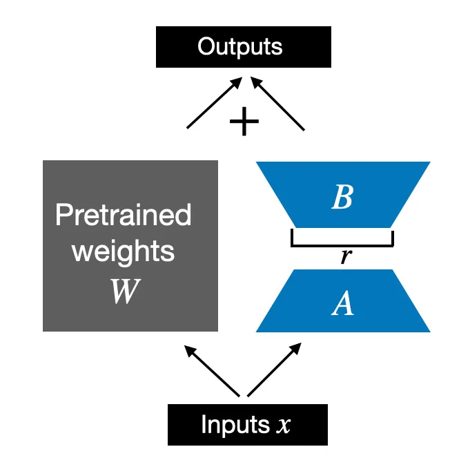
To incorporate the original
Linearlayer weights as shown in the figure above, we implement aLinearWithLoRAlayer below that uses the previously implemented LoRALayer and can be used to replace existingLinearlayers in a neural network, for example, the self-attention module or feed forward modules in an LLM
class LinearWithLoRA(torch.nn.Module):
    def __init__(self, linear, rank, alpha):
        super().__init__()
        self.linear = linear
        self.lora = LoRALayer(
            linear.in_features, linear.out_features, rank, alpha
        )

    def forward(self, x):
        return self.linear(x) + self.lora(x)
Note that since we initialize the weight matrix \(B\) (
self.BinLoRALayer) with zero values in the LoRA layer, the matrix multiplication between \(A\) and \(B\) results in a matrix consisting of 0’s and doesn’t affect the original weights (since adding 0 to the original weights does not modify them)
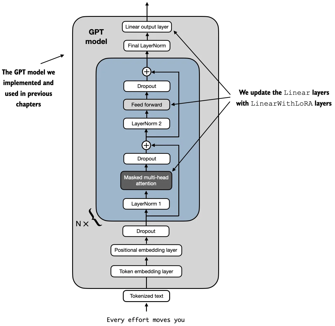
To try LoRA on the GPT model we defined earlier, we define a
replace_linear_with_lorafunction to replace allLinearlayers in the model with the newLinearWithLoRAlayers
def replace_linear_with_lora(model, rank, alpha):
    for name, module in model.named_children():
        if isinstance(module, torch.nn.Linear):
            # Replace the Linear layer with LinearWithLoRA
            setattr(model, name, LinearWithLoRA(module, rank, alpha))
        else:
            # Recursively apply the same function to child modules
            replace_linear_with_lora(module, rank, alpha)
We then freeze the original model parameter and use the
replace_linear_with_lorato replace the saidLinearlayers using the code belowThis will replace the
Linearlayers in the LLM withLinearWithLoRAlayers
total_params = sum(p.numel() for p in model.parameters() if p.requires_grad)
print(f"Total trainable parameters before: {total_params:,}")

for param in model.parameters():
    param.requires_grad = False

total_params = sum(p.numel() for p in model.parameters() if p.requires_grad)
print(f"Total trainable parameters after: {total_params:,}")
Total trainable parameters before: 124,441,346
Total trainable parameters after: 0
replace_linear_with_lora(model, rank=16, alpha=16)

total_params = sum(p.numel() for p in model.parameters() if p.requires_grad)
print(f"Total trainable LoRA parameters: {total_params:,}")
Total trainable LoRA parameters: 2,666,528
As we can see, we reduced the number of trainable parameters by almost 50x when using LoRA
Let’s now double-check whether the layers have been modified as intended by printing the model architecture
device = torch.device("cuda" if torch.cuda.is_available() else "cpu")
model.to(device)

print(model)
GPTModel(
  (tok_emb): Embedding(50257, 768)
  (pos_emb): Embedding(1024, 768)
  (drop_emb): Dropout(p=0.0, inplace=False)
  (trf_blocks): Sequential(
    (0): TransformerBlock(
      (att): MultiHeadAttention(
        (W_query): LinearWithLoRA(
          (linear): Linear(in_features=768, out_features=768, bias=True)
          (lora): LoRALayer()
        )
        (W_key): LinearWithLoRA(
          (linear): Linear(in_features=768, out_features=768, bias=True)
          (lora): LoRALayer()
        )
        (W_value): LinearWithLoRA(
          (linear): Linear(in_features=768, out_features=768, bias=True)
          (lora): LoRALayer()
        )
        (out_proj): LinearWithLoRA(
          (linear): Linear(in_features=768, out_features=768, bias=True)
          (lora): LoRALayer()
        )
        (dropout): Dropout(p=0.0, inplace=False)
      )
      (ff): FeedForward(
        (layers): Sequential(
          (0): LinearWithLoRA(
            (linear): Linear(in_features=768, out_features=3072, bias=True)
            (lora): LoRALayer()
          )
          (1): GELU()
          (2): LinearWithLoRA(
            (linear): Linear(in_features=3072, out_features=768, bias=True)
            (lora): LoRALayer()
          )
        )
      )
      (norm1): LayerNorm()
      (norm2): LayerNorm()
      (drop_resid): Dropout(p=0.0, inplace=False)
    )
    (1): TransformerBlock(
      (att): MultiHeadAttention(
        (W_query): LinearWithLoRA(
          (linear): Linear(in_features=768, out_features=768, bias=True)
          (lora): LoRALayer()
        )
        (W_key): LinearWithLoRA(
          (linear): Linear(in_features=768, out_features=768, bias=True)
          (lora): LoRALayer()
        )
        (W_value): LinearWithLoRA(
          (linear): Linear(in_features=768, out_features=768, bias=True)
          (lora): LoRALayer()
        )
        (out_proj): LinearWithLoRA(
          (linear): Linear(in_features=768, out_features=768, bias=True)
          (lora): LoRALayer()
        )
        (dropout): Dropout(p=0.0, inplace=False)
      )
      (ff): FeedForward(
        (layers): Sequential(
          (0): LinearWithLoRA(
            (linear): Linear(in_features=768, out_features=3072, bias=True)
            (lora): LoRALayer()
          )
          (1): GELU()
          (2): LinearWithLoRA(
            (linear): Linear(in_features=3072, out_features=768, bias=True)
            (lora): LoRALayer()
          )
        )
      )
      (norm1): LayerNorm()
      (norm2): LayerNorm()
      (drop_resid): Dropout(p=0.0, inplace=False)
    )
    (2): TransformerBlock(
      (att): MultiHeadAttention(
        (W_query): LinearWithLoRA(
          (linear): Linear(in_features=768, out_features=768, bias=True)
          (lora): LoRALayer()
        )
        (W_key): LinearWithLoRA(
          (linear): Linear(in_features=768, out_features=768, bias=True)
          (lora): LoRALayer()
        )
        (W_value): LinearWithLoRA(
          (linear): Linear(in_features=768, out_features=768, bias=True)
          (lora): LoRALayer()
        )
        (out_proj): LinearWithLoRA(
          (linear): Linear(in_features=768, out_features=768, bias=True)
          (lora): LoRALayer()
        )
        (dropout): Dropout(p=0.0, inplace=False)
      )
      (ff): FeedForward(
        (layers): Sequential(
          (0): LinearWithLoRA(
            (linear): Linear(in_features=768, out_features=3072, bias=True)
            (lora): LoRALayer()
          )
          (1): GELU()
          (2): LinearWithLoRA(
            (linear): Linear(in_features=3072, out_features=768, bias=True)
            (lora): LoRALayer()
          )
        )
      )
      (norm1): LayerNorm()
      (norm2): LayerNorm()
      (drop_resid): Dropout(p=0.0, inplace=False)
    )
    (3): TransformerBlock(
      (att): MultiHeadAttention(
        (W_query): LinearWithLoRA(
          (linear): Linear(in_features=768, out_features=768, bias=True)
          (lora): LoRALayer()
        )
        (W_key): LinearWithLoRA(
          (linear): Linear(in_features=768, out_features=768, bias=True)
          (lora): LoRALayer()
        )
        (W_value): LinearWithLoRA(
          (linear): Linear(in_features=768, out_features=768, bias=True)
          (lora): LoRALayer()
        )
        (out_proj): LinearWithLoRA(
          (linear): Linear(in_features=768, out_features=768, bias=True)
          (lora): LoRALayer()
        )
        (dropout): Dropout(p=0.0, inplace=False)
      )
      (ff): FeedForward(
        (layers): Sequential(
          (0): LinearWithLoRA(
            (linear): Linear(in_features=768, out_features=3072, bias=True)
            (lora): LoRALayer()
          )
          (1): GELU()
          (2): LinearWithLoRA(
            (linear): Linear(in_features=3072, out_features=768, bias=True)
            (lora): LoRALayer()
          )
        )
      )
      (norm1): LayerNorm()
      (norm2): LayerNorm()
      (drop_resid): Dropout(p=0.0, inplace=False)
    )
    (4): TransformerBlock(
      (att): MultiHeadAttention(
        (W_query): LinearWithLoRA(
          (linear): Linear(in_features=768, out_features=768, bias=True)
          (lora): LoRALayer()
        )
        (W_key): LinearWithLoRA(
          (linear): Linear(in_features=768, out_features=768, bias=True)
          (lora): LoRALayer()
        )
        (W_value): LinearWithLoRA(
          (linear): Linear(in_features=768, out_features=768, bias=True)
          (lora): LoRALayer()
        )
        (out_proj): LinearWithLoRA(
          (linear): Linear(in_features=768, out_features=768, bias=True)
          (lora): LoRALayer()
        )
        (dropout): Dropout(p=0.0, inplace=False)
      )
      (ff): FeedForward(
        (layers): Sequential(
          (0): LinearWithLoRA(
            (linear): Linear(in_features=768, out_features=3072, bias=True)
            (lora): LoRALayer()
          )
          (1): GELU()
          (2): LinearWithLoRA(
            (linear): Linear(in_features=3072, out_features=768, bias=True)
            (lora): LoRALayer()
          )
        )
      )
      (norm1): LayerNorm()
      (norm2): LayerNorm()
      (drop_resid): Dropout(p=0.0, inplace=False)
    )
    (5): TransformerBlock(
      (att): MultiHeadAttention(
        (W_query): LinearWithLoRA(
          (linear): Linear(in_features=768, out_features=768, bias=True)
          (lora): LoRALayer()
        )
        (W_key): LinearWithLoRA(
          (linear): Linear(in_features=768, out_features=768, bias=True)
          (lora): LoRALayer()
        )
        (W_value): LinearWithLoRA(
          (linear): Linear(in_features=768, out_features=768, bias=True)
          (lora): LoRALayer()
        )
        (out_proj): LinearWithLoRA(
          (linear): Linear(in_features=768, out_features=768, bias=True)
          (lora): LoRALayer()
        )
        (dropout): Dropout(p=0.0, inplace=False)
      )
      (ff): FeedForward(
        (layers): Sequential(
          (0): LinearWithLoRA(
            (linear): Linear(in_features=768, out_features=3072, bias=True)
            (lora): LoRALayer()
          )
          (1): GELU()
          (2): LinearWithLoRA(
            (linear): Linear(in_features=3072, out_features=768, bias=True)
            (lora): LoRALayer()
          )
        )
      )
      (norm1): LayerNorm()
      (norm2): LayerNorm()
      (drop_resid): Dropout(p=0.0, inplace=False)
    )
    (6): TransformerBlock(
      (att): MultiHeadAttention(
        (W_query): LinearWithLoRA(
          (linear): Linear(in_features=768, out_features=768, bias=True)
          (lora): LoRALayer()
        )
        (W_key): LinearWithLoRA(
          (linear): Linear(in_features=768, out_features=768, bias=True)
          (lora): LoRALayer()
        )
        (W_value): LinearWithLoRA(
          (linear): Linear(in_features=768, out_features=768, bias=True)
          (lora): LoRALayer()
        )
        (out_proj): LinearWithLoRA(
          (linear): Linear(in_features=768, out_features=768, bias=True)
          (lora): LoRALayer()
        )
        (dropout): Dropout(p=0.0, inplace=False)
      )
      (ff): FeedForward(
        (layers): Sequential(
          (0): LinearWithLoRA(
            (linear): Linear(in_features=768, out_features=3072, bias=True)
            (lora): LoRALayer()
          )
          (1): GELU()
          (2): LinearWithLoRA(
            (linear): Linear(in_features=3072, out_features=768, bias=True)
            (lora): LoRALayer()
          )
        )
      )
      (norm1): LayerNorm()
      (norm2): LayerNorm()
      (drop_resid): Dropout(p=0.0, inplace=False)
    )
    (7): TransformerBlock(
      (att): MultiHeadAttention(
        (W_query): LinearWithLoRA(
          (linear): Linear(in_features=768, out_features=768, bias=True)
          (lora): LoRALayer()
        )
        (W_key): LinearWithLoRA(
          (linear): Linear(in_features=768, out_features=768, bias=True)
          (lora): LoRALayer()
        )
        (W_value): LinearWithLoRA(
          (linear): Linear(in_features=768, out_features=768, bias=True)
          (lora): LoRALayer()
        )
        (out_proj): LinearWithLoRA(
          (linear): Linear(in_features=768, out_features=768, bias=True)
          (lora): LoRALayer()
        )
        (dropout): Dropout(p=0.0, inplace=False)
      )
      (ff): FeedForward(
        (layers): Sequential(
          (0): LinearWithLoRA(
            (linear): Linear(in_features=768, out_features=3072, bias=True)
            (lora): LoRALayer()
          )
          (1): GELU()
          (2): LinearWithLoRA(
            (linear): Linear(in_features=3072, out_features=768, bias=True)
            (lora): LoRALayer()
          )
        )
      )
      (norm1): LayerNorm()
      (norm2): LayerNorm()
      (drop_resid): Dropout(p=0.0, inplace=False)
    )
    (8): TransformerBlock(
      (att): MultiHeadAttention(
        (W_query): LinearWithLoRA(
          (linear): Linear(in_features=768, out_features=768, bias=True)
          (lora): LoRALayer()
        )
        (W_key): LinearWithLoRA(
          (linear): Linear(in_features=768, out_features=768, bias=True)
          (lora): LoRALayer()
        )
        (W_value): LinearWithLoRA(
          (linear): Linear(in_features=768, out_features=768, bias=True)
          (lora): LoRALayer()
        )
        (out_proj): LinearWithLoRA(
          (linear): Linear(in_features=768, out_features=768, bias=True)
          (lora): LoRALayer()
        )
        (dropout): Dropout(p=0.0, inplace=False)
      )
      (ff): FeedForward(
        (layers): Sequential(
          (0): LinearWithLoRA(
            (linear): Linear(in_features=768, out_features=3072, bias=True)
            (lora): LoRALayer()
          )
          (1): GELU()
          (2): LinearWithLoRA(
            (linear): Linear(in_features=3072, out_features=768, bias=True)
            (lora): LoRALayer()
          )
        )
      )
      (norm1): LayerNorm()
      (norm2): LayerNorm()
      (drop_resid): Dropout(p=0.0, inplace=False)
    )
    (9): TransformerBlock(
      (att): MultiHeadAttention(
        (W_query): LinearWithLoRA(
          (linear): Linear(in_features=768, out_features=768, bias=True)
          (lora): LoRALayer()
        )
        (W_key): LinearWithLoRA(
          (linear): Linear(in_features=768, out_features=768, bias=True)
          (lora): LoRALayer()
        )
        (W_value): LinearWithLoRA(
          (linear): Linear(in_features=768, out_features=768, bias=True)
          (lora): LoRALayer()
        )
        (out_proj): LinearWithLoRA(
          (linear): Linear(in_features=768, out_features=768, bias=True)
          (lora): LoRALayer()
        )
        (dropout): Dropout(p=0.0, inplace=False)
      )
      (ff): FeedForward(
        (layers): Sequential(
          (0): LinearWithLoRA(
            (linear): Linear(in_features=768, out_features=3072, bias=True)
            (lora): LoRALayer()
          )
          (1): GELU()
          (2): LinearWithLoRA(
            (linear): Linear(in_features=3072, out_features=768, bias=True)
            (lora): LoRALayer()
          )
        )
      )
      (norm1): LayerNorm()
      (norm2): LayerNorm()
      (drop_resid): Dropout(p=0.0, inplace=False)
    )
    (10): TransformerBlock(
      (att): MultiHeadAttention(
        (W_query): LinearWithLoRA(
          (linear): Linear(in_features=768, out_features=768, bias=True)
          (lora): LoRALayer()
        )
        (W_key): LinearWithLoRA(
          (linear): Linear(in_features=768, out_features=768, bias=True)
          (lora): LoRALayer()
        )
        (W_value): LinearWithLoRA(
          (linear): Linear(in_features=768, out_features=768, bias=True)
          (lora): LoRALayer()
        )
        (out_proj): LinearWithLoRA(
          (linear): Linear(in_features=768, out_features=768, bias=True)
          (lora): LoRALayer()
        )
        (dropout): Dropout(p=0.0, inplace=False)
      )
      (ff): FeedForward(
        (layers): Sequential(
          (0): LinearWithLoRA(
            (linear): Linear(in_features=768, out_features=3072, bias=True)
            (lora): LoRALayer()
          )
          (1): GELU()
          (2): LinearWithLoRA(
            (linear): Linear(in_features=3072, out_features=768, bias=True)
            (lora): LoRALayer()
          )
        )
      )
      (norm1): LayerNorm()
      (norm2): LayerNorm()
      (drop_resid): Dropout(p=0.0, inplace=False)
    )
    (11): TransformerBlock(
      (att): MultiHeadAttention(
        (W_query): LinearWithLoRA(
          (linear): Linear(in_features=768, out_features=768, bias=True)
          (lora): LoRALayer()
        )
        (W_key): LinearWithLoRA(
          (linear): Linear(in_features=768, out_features=768, bias=True)
          (lora): LoRALayer()
        )
        (W_value): LinearWithLoRA(
          (linear): Linear(in_features=768, out_features=768, bias=True)
          (lora): LoRALayer()
        )
        (out_proj): LinearWithLoRA(
          (linear): Linear(in_features=768, out_features=768, bias=True)
          (lora): LoRALayer()
        )
        (dropout): Dropout(p=0.0, inplace=False)
      )
      (ff): FeedForward(
        (layers): Sequential(
          (0): LinearWithLoRA(
            (linear): Linear(in_features=768, out_features=3072, bias=True)
            (lora): LoRALayer()
          )
          (1): GELU()
          (2): LinearWithLoRA(
            (linear): Linear(in_features=3072, out_features=768, bias=True)
            (lora): LoRALayer()
          )
        )
      )
      (norm1): LayerNorm()
      (norm2): LayerNorm()
      (drop_resid): Dropout(p=0.0, inplace=False)
    )
  )
  (final_norm): LayerNorm()
  (out_head): LinearWithLoRA(
    (linear): Linear(in_features=768, out_features=2, bias=True)
    (lora): LoRALayer()
  )
)
Based on the model architecture above, we can see that the model now contains our new
LinearWithLoRAlayersAlso, since we initialized matrix \(B\) with 0’s, we expect the initial model performance to be unchanged compared to before
torch.manual_seed(123)
train_accuracy = calc_accuracy_loader(train_loader, model, device, num_batches=10)
val_accuracy = calc_accuracy_loader(val_loader, model, device, num_batches=10)
test_accuracy = calc_accuracy_loader(test_loader, model, device, num_batches=10)

print(f"Training accuracy: {train_accuracy*100:.2f}%")
print(f"Validation accuracy: {val_accuracy*100:.2f}%")
print(f"Test accuracy: {test_accuracy*100:.2f}%")
Training accuracy: 46.25%
Validation accuracy: 45.00%
Test accuracy: 48.75%
Let’s now get to the interesting part and finetune the model by reusing the training function from chapter 6
The training takes about 15 minutes on a M3 MacBook Air laptop computer and less than half a minute on a V100 or A100 GPU
import time
from previous_chapters import train_classifier_simple
# Alternatively:
# from llms_from_scratch.ch06 import train_classifier_simple


start_time = time.time()

torch.manual_seed(123)

optimizer = torch.optim.AdamW(model.parameters(), lr=5e-5, weight_decay=0.1)

num_epochs = 5
train_losses, val_losses, train_accs, val_accs, examples_seen = train_classifier_simple(
    model, train_loader, val_loader, optimizer, device,
    num_epochs=num_epochs, eval_freq=50, eval_iter=5,
)

end_time = time.time()
execution_time_minutes = (end_time - start_time) / 60
print(f"Training completed in {execution_time_minutes:.2f} minutes.")
Ep 1 (Step 000000): Train loss 3.820, Val loss 3.462
Ep 1 (Step 000050): Train loss 0.396, Val loss 0.364
Ep 1 (Step 000100): Train loss 0.111, Val loss 0.229
Training accuracy: 97.50% | Validation accuracy: 95.00%
Ep 2 (Step 000150): Train loss 0.135, Val loss 0.073
Ep 2 (Step 000200): Train loss 0.008, Val loss 0.052
Ep 2 (Step 000250): Train loss 0.021, Val loss 0.179
Training accuracy: 97.50% | Validation accuracy: 97.50%
Ep 3 (Step 000300): Train loss 0.096, Val loss 0.080
Ep 3 (Step 000350): Train loss 0.010, Val loss 0.116
Training accuracy: 97.50% | Validation accuracy: 95.00%
Ep 4 (Step 000400): Train loss 0.003, Val loss 0.151
Ep 4 (Step 000450): Train loss 0.008, Val loss 0.077
Ep 4 (Step 000500): Train loss 0.001, Val loss 0.147
Training accuracy: 100.00% | Validation accuracy: 97.50%
Ep 5 (Step 000550): Train loss 0.007, Val loss 0.094
Ep 5 (Step 000600): Train loss 0.000, Val loss 0.056
Training accuracy: 100.00% | Validation accuracy: 97.50%
Training completed in 12.10 minutes.
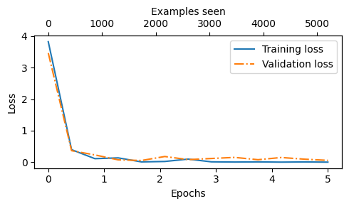
Finally, let’s evaluate the model
from previous_chapters import plot_values
# Alternatively:
# from llms_from_scratch.ch06 import plot_values

epochs_tensor = torch.linspace(0, num_epochs, len(train_losses))
examples_seen_tensor = torch.linspace(0, examples_seen, len(train_losses))

plot_values(epochs_tensor, examples_seen_tensor, train_losses, val_losses, label="loss")
Note that we previously calculated the accuracy values on 5 batches only via the
eval_iter=5setting; below, we calculate the accuracies on the full dataset
train_accuracy = calc_accuracy_loader(train_loader, model, device)
val_accuracy = calc_accuracy_loader(val_loader, model, device)
test_accuracy = calc_accuracy_loader(test_loader, model, device)

print(f"Training accuracy: {train_accuracy*100:.2f}%")
print(f"Validation accuracy: {val_accuracy*100:.2f}%")
print(f"Test accuracy: {test_accuracy*100:.2f}%")
Training accuracy: 100.00%
Validation accuracy: 96.64%
Test accuracy: 97.33%
As we can see based on the relatively high accuracy values above, the LoRA finetuning was successful