|
Supplementary code for the Build a Large Language Model From Scratch book by Sebastian Raschka Code repository: https://github.com/rasbt/LLMs-from-scratch |

|
Understanding the Difference Between Embedding Layers and Linear Layers#
Embedding layers in PyTorch accomplish the same as linear layers that perform matrix multiplications; the reason we use embedding layers is computational efficiency
We will take a look at this relationship step by step using code examples in PyTorch
import torch

print("PyTorch version:", torch.__version__)
---------------------------------------------------------------------------
ModuleNotFoundError                       Traceback (most recent call last)
Cell In[1], line 1
----> 1 import torch
      3 print("PyTorch version:", torch.__version__)

ModuleNotFoundError: No module named 'torch'
Using nn.Embedding#
# Suppose we have the following 3 training examples,
# which may represent token IDs in a LLM context
idx = torch.tensor([2, 3, 1])

# The number of rows in the embedding matrix can be determined
# by obtaining the largest token ID + 1.
# If the highest token ID is 3, then we want 4 rows, for the possible
# token IDs 0, 1, 2, 3
num_idx = max(idx)+1

# The desired embedding dimension is a hyperparameter
out_dim = 5
Let’s implement a simple embedding layer:
# We use the random seed for reproducibility since
# weights in the embedding layer are initialized with
# small random values
torch.manual_seed(123)

embedding = torch.nn.Embedding(num_idx, out_dim)
We can optionally take a look at the embedding weights:
embedding.weight
Parameter containing:
tensor([[ 0.3374, -0.1778, -0.3035, -0.5880,  1.5810],
        [ 1.3010,  1.2753, -0.2010, -0.1606, -0.4015],
        [ 0.6957, -1.8061, -1.1589,  0.3255, -0.6315],
        [-2.8400, -0.7849, -1.4096, -0.4076,  0.7953]], requires_grad=True)
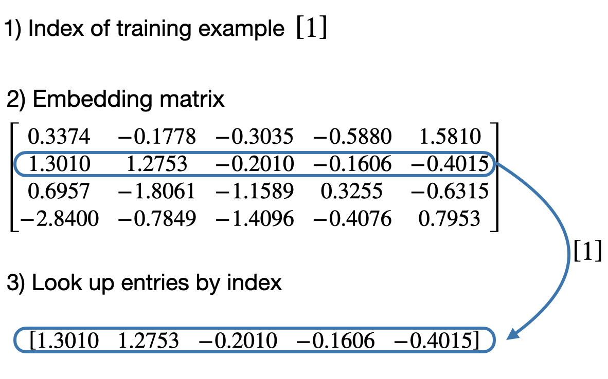
We can then use the embedding layers to obtain the vector representation of a training example with ID 1:
embedding(torch.tensor([1]))
tensor([[ 1.3010,  1.2753, -0.2010, -0.1606, -0.4015]],
       grad_fn=<EmbeddingBackward0>)
Below is a visualization of what happens under the hood:
Similarly, we can use embedding layers to obtain the vector representation of a training example with ID 2:
embedding(torch.tensor([2]))
tensor([[ 0.6957, -1.8061, -1.1589,  0.3255, -0.6315]],
       grad_fn=<EmbeddingBackward0>)

Now, let’s convert all the training examples we have defined previously:
idx = torch.tensor([2, 3, 1])
embedding(idx)
tensor([[ 0.6957, -1.8061, -1.1589,  0.3255, -0.6315],
        [-2.8400, -0.7849, -1.4096, -0.4076,  0.7953],
        [ 1.3010,  1.2753, -0.2010, -0.1606, -0.4015]],
       grad_fn=<EmbeddingBackward0>)
Under the hood, it’s still the same look-up concept:

Using nn.Linear#
Now, we will demonstrate that the embedding layer above accomplishes exactly the same as
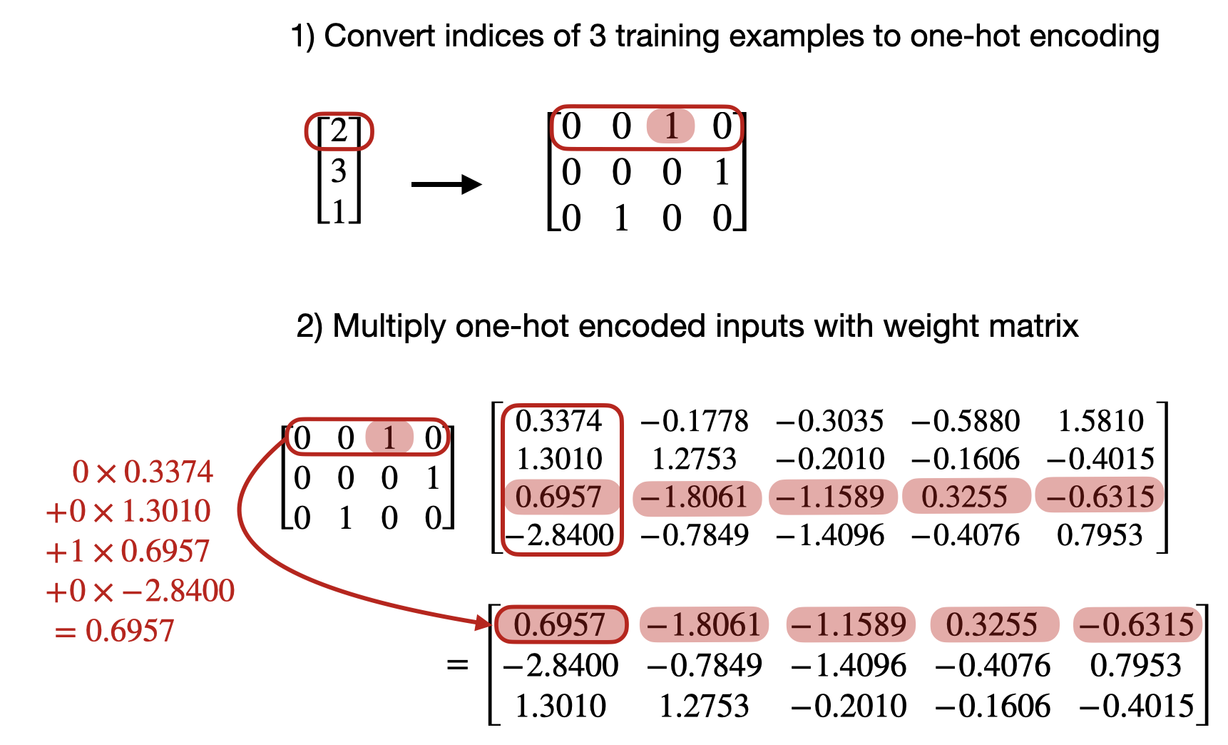
nn.Linearlayer on a one-hot encoded representation in PyTorchFirst, let’s convert the token IDs into a one-hot representation:
onehot = torch.nn.functional.one_hot(idx)
onehot
tensor([[0, 0, 1, 0],
        [0, 0, 0, 1],
        [0, 1, 0, 0]])
Next, we initialize a
Linearlayer, which carries out a matrix multiplication \(X W^\top\):
torch.manual_seed(123)
linear = torch.nn.Linear(num_idx, out_dim, bias=False)
linear.weight
Parameter containing:
tensor([[-0.2039,  0.0166, -0.2483,  0.1886],
        [-0.4260,  0.3665, -0.3634, -0.3975],
        [-0.3159,  0.2264, -0.1847,  0.1871],
        [-0.4244, -0.3034, -0.1836, -0.0983],
        [-0.3814,  0.3274, -0.1179,  0.1605]], requires_grad=True)
Note that the linear layer in PyTorch is also initialized with small random weights; to directly compare it to the
Embeddinglayer above, we have to use the same small random weights, which is why we reassign them here:
linear.weight = torch.nn.Parameter(embedding.weight.T)
Now we can use the linear layer on the one-hot encoded representation of the inputs:
linear(onehot.float())
tensor([[ 0.6957, -1.8061, -1.1589,  0.3255, -0.6315],
        [-2.8400, -0.7849, -1.4096, -0.4076,  0.7953],
        [ 1.3010,  1.2753, -0.2010, -0.1606, -0.4015]], grad_fn=<MmBackward0>)
As we can see, this is exactly the same as what we got when we used the embedding layer:
embedding(idx)
tensor([[ 0.6957, -1.8061, -1.1589,  0.3255, -0.6315],
        [-2.8400, -0.7849, -1.4096, -0.4076,  0.7953],
        [ 1.3010,  1.2753, -0.2010, -0.1606, -0.4015]],
       grad_fn=<EmbeddingBackward0>)
What happens under the hood is the following computation for the first training example’s token ID:
And for the second training example’s token ID:
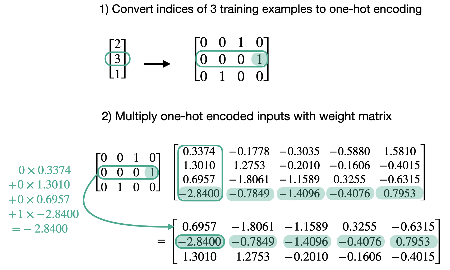
Since all but one index in each one-hot encoded row are 0 (by design), this matrix multiplication is essentially the same as a look-up of the one-hot elements
This use of the matrix multiplication on one-hot encodings is equivalent to the embedding layer look-up but can be inefficient if we work with large embedding matrices, because there are a lot of wasteful multiplications by zero